A journey from dataset acquisition to live webcam inference using deep learning.

Source: github.com/brianhliou/happy-face

Introduction

Human facial expressions are a fundamental part of non-verbal communication. In this project, I built a deep learning system that recognizes seven basic emotions in real-time using a webcam. This blog post walks through the entire process: from setting up the project structure, training a custom CNN on the FER-2013 dataset, to achieving 59% validation accuracy and deploying a live inference system.

Tech Stack: Python, TensorFlow, Keras, OpenCV, NumPy

Project Overview

The goal was to create an end-to-end facial expression recognition system that could:

1. Train a model to classify 7 emotions: Angry, Disgust, Fear, Happy, Neutral, Sad, Surprise
2. Generate comprehensive training reports with metrics and visualizations
3. Perform real-time inference using a webcam feed
4. Provide smooth, user-friendly predictions

Final Results: 59.3% validation accuracy on FER-2013, with strong performance on Happy (86% precision) and Surprise (82% recall).

Dataset: FER-2013

The FER-2013 (Facial Expression Recognition 2013) dataset is a popular benchmark for facial expression recognition:

• Size: 35,887 grayscale images
• Split: 28,709 training, 7,178 validation
• Resolution: 48×48 pixels
• Classes: 7 emotions
• Challenge: Highly imbalanced (Happy: 8,989 images vs Disgust: 547 images)

Model Architecture

I designed a custom Convolutional Neural Network (CNN) optimized for the small 48×48 input size. Let me break down how it works.

Understanding Convolutional Neural Networks

CNNs are designed to process grid-like data (images) by learning hierarchical features:

Early layers detect simple patterns:

• Edges (horizontal, vertical, diagonal)
• Textures and gradients
• Basic shapes

Middle layers combine these into:

• Facial features (eyes, nose, mouth)
• Facial contours
• Expression-specific patterns

Deep layers recognize:

• Complete facial expressions
• Emotion-specific configurations
• Context and relationships

Network Architecture

My model uses 4 convolutional blocks followed by 2 dense layers:

Input: 48×48 grayscale image
    ↓
[Conv Block 1]
  64 filters (3×3) → Find basic edges and textures
  BatchNorm       → Stabilize learning
  ReLU           → Add non-linearity
  MaxPool (2×2)  → Reduce to 24×24
  Dropout (25%)  → Prevent overfitting
    ↓
[Conv Block 2]
  128 filters (5×5) → Combine edges into facial features
  BatchNorm
  ReLU
  MaxPool (2×2)   → Reduce to 12×12
  Dropout (25%)
    ↓
[Conv Block 3]
  512 filters (3×3) → Detect complex patterns
  BatchNorm
  ReLU
  MaxPool (2×2)   → Reduce to 6×6
  Dropout (25%)
    ↓
[Conv Block 4]
  512 filters (3×3) → Recognize full expressions
  BatchNorm
  ReLU
  MaxPool (2×2)   → Reduce to 3×3
  Dropout (25%)
    ↓
Flatten: 3×3×512 = 4,608 features
    ↓
[Dense Layer 1]
  256 neurons → Compress features
  BatchNorm
  ReLU
  Dropout (25%)
    ↓
[Dense Layer 2]
  512 neurons → Learn emotion combinations
  BatchNorm
  ReLU
  Dropout (25%)
    ↓
[Output Layer]
  7 neurons (Softmax) → Final emotion probabilities

Total Parameters: ~4.5 million trainable weights

Why This Architecture?

1. Progressive Complexity: Filter count increases (64→128→512→512) as we move deeper, allowing the network to learn increasingly abstract representations

2. Batch Normalization: Normalizes activations between layers, making training more stable and allowing higher learning rates

3. Dropout (25%): Randomly “turns off” 25% of neurons during training, forcing the network to learn robust features instead of memorizing training data

4. MaxPooling: Reduces spatial dimensions while retaining important features, making the model translation-invariant (recognizes expressions regardless of exact face position)

5. Dual Dense Layers: Two fully-connected layers (256→512) before output allow the model to learn complex combinations of features for emotion classification

What Happens During Training?

Training a neural network involves repeatedly showing it examples and adjusting its weights to minimize mistakes. Here’s the step-by-step process:

1. Forward Pass (Making Predictions)

For each training image:

1. Input: Feed a 48×48 grayscale face image into the network
2. Convolution: Each convolutional layer applies learned filters to detect patterns
3. Activation: ReLU function adds non-linearity (allows learning complex patterns)
4. Pooling: Reduces size while keeping important information
5. Dense Layers: Combine all learned features
6. Output: Softmax produces 7 probabilities (one per emotion)

Example output: [Angry: 0.05, Disgust: 0.02, Fear: 0.03, Happy: 0.78, Neutral: 0.06, Sad: 0.04, Surprise: 0.02]

2. Calculate Loss (How Wrong Were We?)

The model compares its prediction to the true label using Categorical Cross-Entropy Loss:

True label: Happy (index 3)
Prediction: [0.05, 0.02, 0.03, 0.78, 0.06, 0.04, 0.02]
Loss: -log(0.78) = 0.25  # Lower is better

Good prediction (high confidence in correct class) = Low loss
Bad prediction (low confidence in correct class) = High loss

3. Backward Pass (Learning from Mistakes)

This is where the magic happens:

1. Compute Gradients: Calculate how much each weight contributed to the error
2. Backpropagation: Work backwards through the network, layer by layer
3. Update Weights: Adjust all 4.5 million parameters slightly to reduce loss

The Adam optimizer determines how much to adjust each weight:

• Larger gradients = bigger updates
• Adaptive learning rates for each parameter
• Momentum to escape local minima

4. Repeat for Entire Dataset (1 Epoch)

One epoch = seeing all 28,709 training images once:

• Process in batches of 64 images (448 batches per epoch)
• Update weights after each batch
• Track training accuracy and loss

5. Validation (Check Generalization)

After each epoch:

1. Run the model on 7,178 validation images (never seen during training)
2. Calculate validation accuracy and loss
3. Key insight: If validation accuracy improves, the model is learning generalizable patterns. If it decreases, we’re overfitting.

6. Training Dynamics

During my 50-epoch training run, three callbacks managed the training process automatically:

• ModelCheckpoint saved the model only when validation accuracy improved (13 times total)
• ReduceLROnPlateau reduced learning rate when progress stalled (activated around epoch 19)
• EarlyStopping would halt training after 10 epochs without improvement (never triggered)

Additionally, class weighting penalized mistakes on rare emotions (Disgust) more heavily than common ones (Happy).

Here’s what actually happened during training:

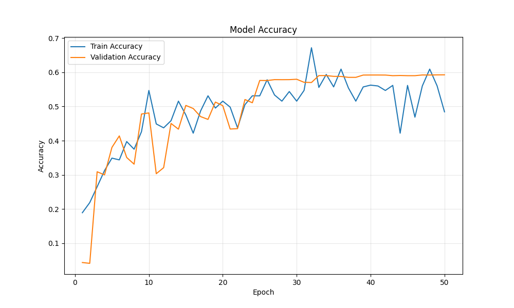Training and validation accuracy over 50 epochs

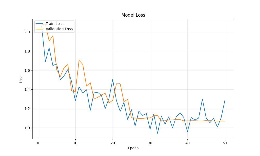Loss decreased smoothly, showing effective learning

Key observations:

• Training accuracy: 17% → 53%
• Validation accuracy: 31% → 59%
• No overfitting (validation tracked training closely)
• Learning rate reduction at epoch ~19 provided a slight boost

Training Process

Data Augmentation

To improve generalization, I applied real-time data augmentation:

- Rotation: ±20 degrees
- Width/Height Shift: ±20%
- Horizontal Flip: 50% chance
- Zoom: ±20%

This artificially expanded the training set and helped the model learn rotation and position-invariant features.

Handling Class Imbalance

The FER-2013 dataset has significant class imbalance. To address this, I implemented class weighting:

class_weights = {
    0: 1.03,   # Angry
    1: 9.41,   # Disgust - heavily weighted due to scarcity
    2: 1.00,   # Fear
    3: 0.57,   # Happy - downweighted due to abundance
    4: 0.83,   # Neutral
    5: 0.85,   # Sad
    6: 1.29    # Surprise
}

This forces the model to pay more attention to rare classes during training.

Training Configuration

• Optimizer: Adam (adaptive learning rate)
• Loss Function: Categorical Cross-Entropy
• Initial Learning Rate: 0.001
• Batch Size: 64
• Epochs: 50

Final Training Results

Training Time: ~49 minutes (50 epochs on M-series Mac CPU)

The model achieved its best validation accuracy of 59.3% at epoch 50, showing continuous improvement throughout training without overfitting.

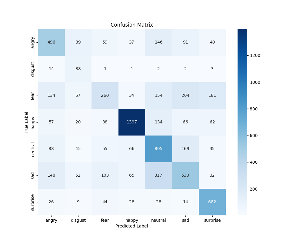Confusion matrix showing which emotions are commonly confused

Performance Metrics

Emotion	Precision	Recall	F1-Score	Support
Angry	0.52	0.52	0.52	958
Disgust	0.27	0.79	0.40	111
Fear	0.46	0.25	0.33	1024
Happy	0.86	0.79	0.82	1774
Neutral	0.51	0.65	0.57	1233
Sad	0.49	0.43	0.46	1247
Surprise	0.66	0.82	0.73	831

Key Observations:

• Happy performed best (82% F1-score) - likely due to abundant training data and distinct facial features
• Surprise showed high recall (82%) - the model rarely misses surprised faces
• Disgust struggled with precision (27%) despite class weighting - very limited training data (111 samples)
• Fear had low recall (25%) - often confused with sadness or surprise

Real-Time Inference System

The final step was deploying the model for real-time webcam inference.

Implementation

The inference pipeline consists of:

1. Face Detection: OpenCV’s Haar Cascade classifier detects faces in each frame
2. Preprocessing:
   • Convert to grayscale
   • Resize to 48×48
   • Normalize pixel values to [0, 1]
3. Prediction: Feed into the trained CNN
4. Display: Show bounding box, emotion label, and confidence

Smoothing Techniques

Initial implementation had severe flickering due to inconsistent frame-by-frame face detection. I implemented several smoothing techniques:

Prediction Persistence (15 frames):

• Keep the last valid prediction visible for ~0.5 seconds
• Prevents UI from jumping between “face detected” and “no face”

Frame Skipping (every 2nd frame):

• Run detection only every 2 frames for performance
• Reduces computational load and jitter

Lenient Detection Parameters:

scaleFactor=1.1  # More sensitive to faces
minNeighbors=4   # Accept faces with fewer confirming detections
minSize=(30, 30) # Smaller minimum face size

User Interface

The inference window shows:

• Left Panel: Live webcam feed with bounding boxes and emotion labels
• Right Panel:
  • Preprocessed 48×48 grayscale image (what the model sees)
  • Probability bars for all 7 emotions
  • Highlighted prediction with confidence percentage

Example Predictions:

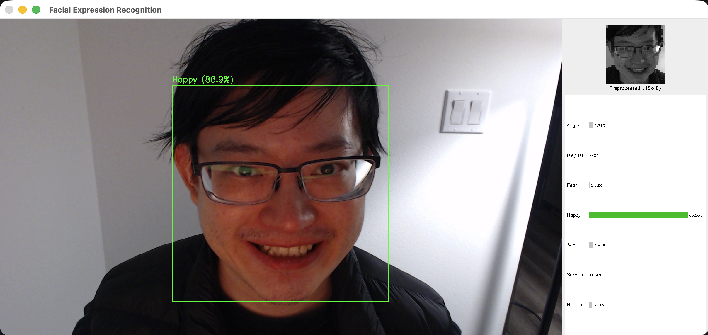Detecting happiness with 88.9% confidence

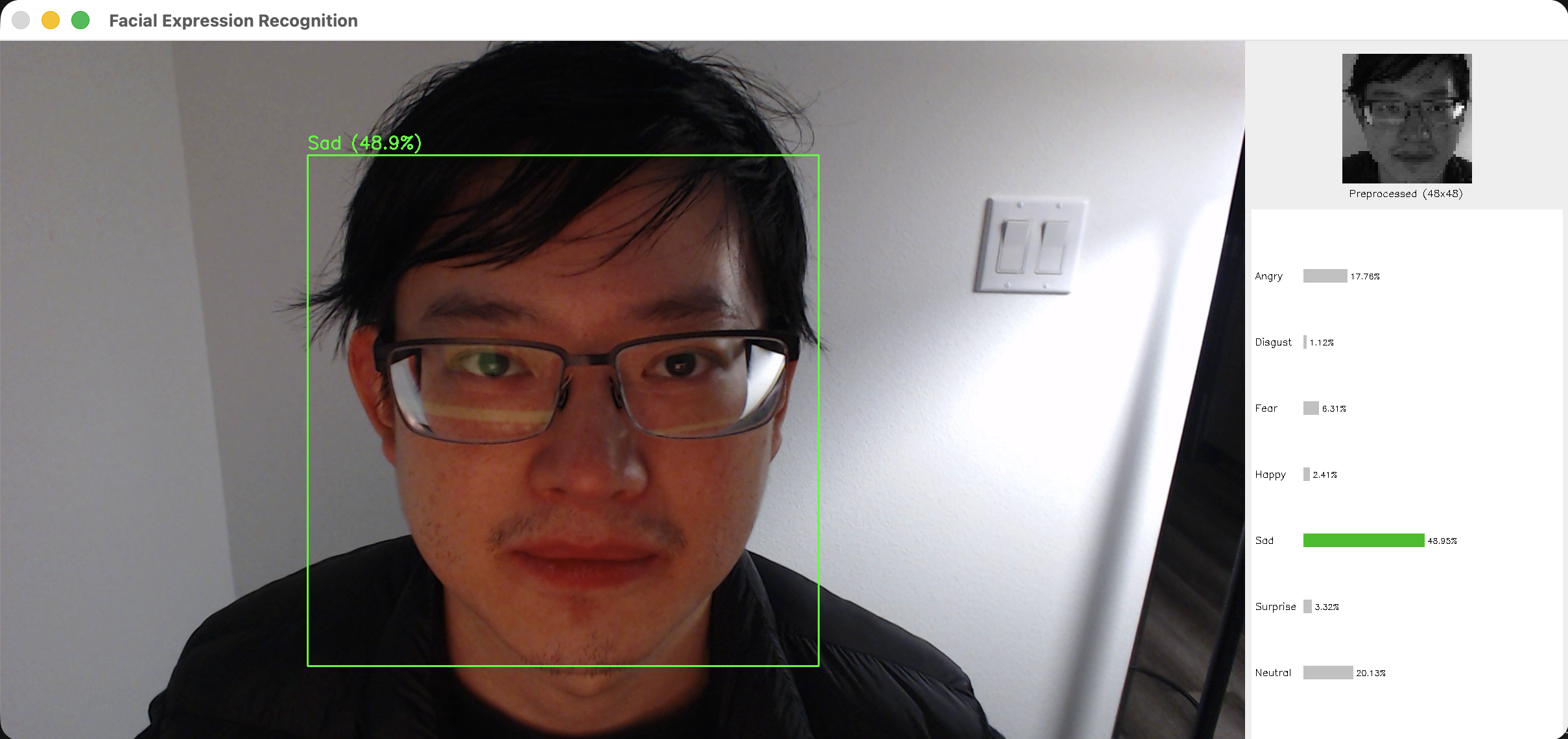Detecting sadness with 48.9% confidence

The split-screen UI makes it easy to see both what the camera captures and what the model actually “sees” (the preprocessed 48×48 grayscale image), helping users understand the preprocessing pipeline.

Challenges and Solutions

Challenge 1: Class Imbalance

Problem: Disgust had only 547 images vs Happy’s 8,989 Solution: Implemented class weighting during training to penalize mistakes on rare classes more heavily

Challenge 2: Low Resolution

Problem: 48×48 pixels is very small - many facial details are lost
Solution: Used aggressive data augmentation and multiple convolutional layers to extract maximum information

Challenge 3: Real-Time Flickering

Problem: Face detection was inconsistent frame-to-frame, causing jarring UI updates
Solution: Added prediction persistence and frame skipping for smooth, readable predictions

Challenge 4: Camera Compatibility

Problem: OpenCV couldn’t read from external USB webcam (C922)
Solution: Tested multiple camera indices and added automatic fallback to built-in camera

Lessons Learned

1. Data Quality Matters: The model performed best on emotions with clean, abundant training data (Happy, Surprise)
2. Regularization is Critical: Without Batch Normalization and Dropout, the model quickly overfitted
3. User Experience != Model Accuracy: A 59% accurate model with smooth, persistent predictions feels better than a 70% model that flickers constantly
4. Callbacks Save Time: Early stopping prevented wasted training time; ReduceLROnPlateau helped squeeze out extra accuracy

Future Improvements

1. Transfer Learning: Use pre-trained models (ResNet, EfficientNet) for better feature extraction
2. Ensemble Methods: Combine multiple models for improved accuracy
3. Better Dataset: FER-2013 has noisy labels; newer datasets (AffectNet, RAF-DB) could improve performance
4. Attention Mechanisms: Focus model on key facial regions (eyes, mouth)
5. Web Deployment: Package as a Flask/FastAPI app for browser-based demos

Conclusion

This project demonstrated the complete lifecycle of a deep learning application - from data acquisition and model training to real-world deployment. While 59% accuracy might seem modest, it’s competitive with published baselines on FER-2013 and works surprisingly well in practice for clear, well-lit facial expressions.

The real-time inference system successfully bridges the gap between a trained model and a usable product, emphasizing the importance of user experience alongside model performance.

Code Available: GitHub Repository

---

Technologies: Python 3.9, TensorFlow 2.x, Keras, OpenCV, NumPy, Matplotlib
Training Hardware: M-series Mac (CPU training)
Dataset: FER-2013 (Kaggle)