Gobblet Gobblers is a tic-tac-toe variant with a stacking mechanic, marketed as a children’s game (ages 5+). I solved the game, built a 20-million position tablebase, and deployed a web UI for exploring optimal play.

Result: Player 1 wins with perfect play.

This post covers the solver implementation, the 180× Rust rewrite, and the deployment architecture.

Demo: gobblet-gobblers-tablebase.vercel.app
Source: github.com/brianhliou/gobblet-gobblers

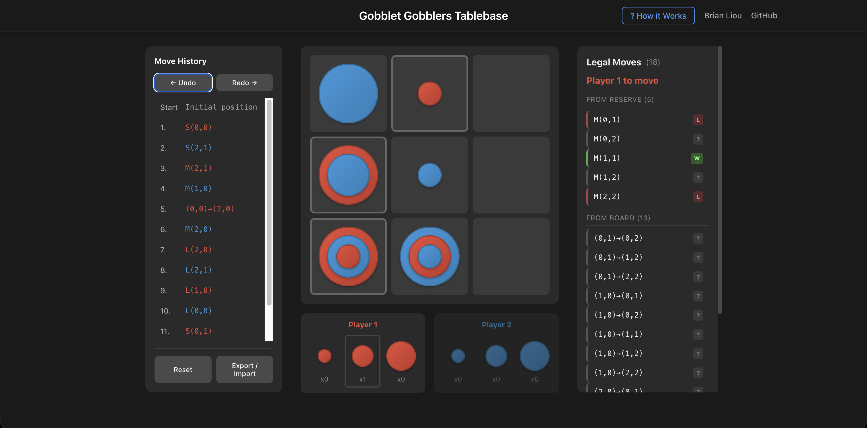The analysis interface showing move evaluations. Green indicates winning moves, red indicates losing moves.

---

1. Game Rules

Gobblet Gobblers is a two-player game on a 3×3 board. Each player has six pieces: two small, two medium, and two large. Victory requires placing three pieces of your color in a row (horizontal, vertical, or diagonal).

Initial position

Red large gobbles blue small

The distinguishing mechanic is gobbling: larger pieces can cover smaller pieces of either color. When a large piece is placed on top of a small piece, the small piece becomes hidden and does not count toward winning lines. Only the top piece of each stack is visible.

The reveal rule introduces significant complexity. When a player lifts a piece to move it, any piece underneath becomes visible. If this reveals an opponent’s winning line, the moving player loses, unless the piece being moved can legally gobble one of the pieces in that winning line. This “hail mary” escape is the only recourse.

P2's large hides P1's small

P2 gobbles into column 0 to survive

Several edge cases arise from this rule:

1. Simultaneous reveal and win: If your move creates your own three-in-a-row while also revealing the opponent’s winning line, the reveal takes precedence: the lift happens before the place. You lose.

2. Same-square restriction: A piece cannot be placed back on the square it was lifted from. If the only valid gobble target is the origin square, there is no legal escape.

3. Multiple revealed lines: If lifting reveals two or more winning lines, blocking all of them with a single piece is typically impossible.

4. Zugzwang: If a player has no legal moves (all possible piece lifts would reveal opponent wins with no valid escape), that player loses immediately.

The game ends in a draw upon threefold repetition of the same board position.

---

2. Results

Primary Finding

Player 1 (first mover) wins with optimal play.

This was determined through minimax search with alpha-beta pruning.

Important Limitations

This is not an exhaustive solve. Alpha-beta pruning, by design, skips branches once a winning move is found. The 19,836,040 positions in the tablebase represent the positions visited during our search, not the complete set of reachable positions.

The solution proves P1 can force a win, but:

1. Not necessarily optimal. Move ordering prioritized smaller pieces before larger ones to improve pruning efficiency. The solver found that P1 wins by leading with small piece placements, but this may not be the shortest path to victory. A different move ordering might discover a faster win.

2. Not exhaustive. When the solver found a winning move at a P1-to-move position, it stopped searching other moves from that position. Those unexplored branches may contain positions not in our tablebase. At P2-to-move positions, all moves were explored (P2 must check every escape attempt), so P2’s options are complete.

3. Tablebase coverage is path-dependent. The 19.8M positions reflect what our specific search order encountered.

Tablebase Statistics

Statistics for positions visited during our alpha-beta search:

Metric	Value
Positions in tablebase	19,836,040
P1 winning positions	10,226,838 (51.56%)
P2 winning positions	9,570,219 (48.25%)
Drawn positions	38,983 (0.20%)

The low draw rate (0.20%) among visited positions is notable.

Note: These percentages describe the visited positions, not the full game. The complete state space is ~341 million positions; our pruned search visited only ~20 million of them.

Game Length

Optimal play: P1 wins in 13 plies (7 moves).

With optimal play by both sides, P1 forces a win in 13 plies. The winning first move is a small or large piece; opening with a medium piece is a mistake.

---

3. Approach

Algorithm

The solver uses minimax search with alpha-beta pruning and transposition tables.

Minimax computes the outcome of a position recursively: a position is winning for the current player if any child position is losing for the opponent; losing if all children are winning for the opponent; drawn otherwise.

Alpha-beta pruning eliminates branches that cannot affect the final result. If the maximizing player has already found a winning move, remaining moves need not be evaluated. This optimization is only effective when good moves are explored first.

Transposition tables cache position outcomes to avoid redundant computation when the same position is reachable via different move sequences.

Symmetry Reduction

The 3×3 board has D₄ symmetry (8 equivalent configurations under rotation and reflection). Before lookup or storage, positions are canonicalized by computing all 8 transformations and selecting the lexicographically smallest encoding.

Identity

Rotate 90°

Rotate 180°

Rotate 270°

Flip H

Flip V

Flip diag

Flip anti-diag

Transformations:
- Identity
- Rotate 90° CW
- Rotate 180°
- Rotate 270° CW
- Reflect horizontal
- Reflect vertical
- Reflect main diagonal
- Reflect anti-diagonal

This reduces the effective state space by approximately 8× for most positions (some positions are self-symmetric).

Tablebase Construction

The goal is a mapping from canonical position hash to outcome. Given this tablebase, optimal play reduces to: look up the current position, enumerate legal moves, look up each resulting position, choose any move that preserves your winning status (or minimizes loss).

---

4. Implementation: V1 (Python)

Initial Design

The first implementation used an object-oriented design in Python. GameState objects encapsulated board state, reserves, and current player. Piece objects represented individual pieces with player and size attributes. Move generation returned Move objects.

To explore a child position, the solver deep-copied the current state, applied the move to the copy, recursed, then discarded the copy.

This design was correct but exhibited unacceptable performance.

Performance Analysis

Benchmarking revealed the bottleneck:

Operation	Time per position
generate_moves()	18 µs
play_move() × 27 moves	567 µs
└─ deepcopy() overhead	420 µs (75%)
encode_state() × 27	40 µs
canonicalize() × 27	222 µs
Total	~850 µs

deepcopy consumed 75% of play_move time, approximately 15 µs per copy, 27 copies per position. At 750 positions/second, solving would require days.

Additionally, Python’s default recursion limit (~10,000) was insufficient. The game tree extends to depths exceeding 400 moves. The solver was converted to an iterative implementation using an explicit stack of StackFrame objects.

Optimization: Undo-Based Move Application

Rather than copy-mutate-discard, the optimized approach mutates in place and undoes the mutation when backtracking:

# Before: copy-based (slow)
child_state = state.copy()  # Deep copy
apply_move(child_state, move)
outcome = solve(child_state)

# After: undo-based (fast)
undo_info = apply_move_in_place(state, move)  # Mutate directly
outcome = solve(state)
undo_move_in_place(state, undo_info)  # Restore

This required tracking sufficient information to reverse each move: which piece was captured at the destination, which piece was revealed at the source, whether the player turn was switched.

Result: 750 → 2,000 positions/second (2.7× speedup).

Optimization: Disabling Garbage Collection

During enumeration, progress stopped entirely at ~70 million objects in memory. Profiling revealed Python’s cyclic garbage collector was scanning all objects to find reference cycles:

815/817 samples in _PyGC_Collect → mark_all_reachable

With tens of millions of objects (26M in one dict, 24M in another set, 20M in the transposition table), each GC scan consumed minutes. The data structures contained only integers, so no reference cycles were possible.

Fix: gc.disable() during hot loops. Reference counting (non-cyclic cleanup) continues to function.

Optimization: Shared Path Set

Each StackFrame initially stored a frozenset of all positions on the current path for cycle detection. At depth D, frame D contains a frozenset of D elements. Total storage: O(D²).

At depth 84,000:

1 + 2 + ... + 84,000 = 3.5 billion integers across frames

Fix: Use a single shared set for the entire search. Add positions when pushing frames, remove when popping. Storage: O(D).

Final Python Performance

With all optimizations (undo-based moves, gc.disable, shared path set), throughput reached ~3,700 positions/second. Total solve time: 1.5 hours.

---

5. Implementation: V2 (Rust)

Motivation

3,700 positions/second was sufficient to complete the solve, but a Rust rewrite offered both performance gains and a verification opportunity: two independent implementations should produce identical results.

Why Rust

The Python bottlenecks pointed directly at language-level constraints:

1. Object overhead. Python objects carry type information, reference counts, and GC metadata. A simple Piece(player=1, size=2) occupies ~100 bytes. In Rust, this is 2 bytes (or 1 byte with packing).

2. Garbage collection. Even with gc.disable(), Python’s reference counting still runs on every object creation and destruction. Rust has no runtime GC; memory is managed at compile time.

3. Heap allocation. Python allocates nearly everything on the heap. Rust allows stack allocation for fixed-size data, avoiding allocator overhead entirely.

4. Memory layout control. Python dictionaries and lists have indirection and padding. Rust’s #[repr(packed)] and bitfield operations allow exact control over memory layout.

The bit-packed representation described below is technically possible in Python (using integers as bitfields), but the surrounding code would still pay Python’s interpretation overhead. Rust compiles these bit operations to native instructions.

Bit-Level Encoding

The V2 representation eliminates all object allocation in the hot path:

Board state (64 bits): The entire game state fits in a single u64.

Bits 0-53:  Board (9 cells × 6 bits)
Bit 54:     Current player (0=P1, 1=P2)
Bits 55-63: Unused

Cell encoding (6 bits):
  Bits 0-1: Small piece owner  (0=empty, 1=P1, 2=P2)
  Bits 2-3: Medium piece owner
  Bits 4-5: Large piece owner

Each cell can hold at most one piece of each size (the stacking constraint). With 3 sizes × 2 bits per size = 6 bits per cell, 9 cells × 6 bits = 54 bits for the full board.

Move encoding (8 bits): PackedMove is a single byte.

Bits 0-3: Destination (0-8)
Bits 4-7: Source (0-8 for slides, 9-11 for reserve placement by size)

Undo encoding (16 bits): PackedUndo stores the move plus captured/revealed pieces.

Bits 0-7:   PackedMove
Bits 8-10:  Captured piece (3-bit encoding)
Bits 11-13: Revealed piece (3-bit encoding)

Win detection (bitmask): Precomputed masks for the 8 winning lines enable branchless checking:

const WIN_MASKS: [u16; 8] = [
    0b000_000_111, // Row 0
    0b000_111_000, // Row 1
    0b111_000_000, // Row 2
    0b001_001_001, // Col 0
    0b010_010_010, // Col 1
    0b100_100_100, // Col 2
    0b100_010_001, // Main diagonal
    0b001_010_100, // Anti-diagonal
];

fn check_winner(&self) -> Option<Player> {
    let (p1_mask, p2_mask) = self.visibility_masks();
    for &win in &WIN_MASKS {
        if (p1_mask & win) == win { return Some(Player::One); }
        if (p2_mask & win) == win { return Some(Player::Two); }
    }
    None
}

Memory Comparison

Component	Python V1	Rust V2
Board state	~500 bytes (objects + GC overhead)	8 bytes (u64)
Move	~100 bytes	1 byte (u8)
Undo info	~200 bytes	2 bytes (u16)
Move list	Heap allocation	Stack-allocated

Performance Result

Metric	Python V1	Rust V2	Improvement
Solve time	1.5 hours	31 seconds	174×
Positions/sec	~3,700	~640,000	173×

The Rust solver evaluated 19,836,040 unique positions. The ~180× speedup comes entirely from eliminating allocation overhead and using compact representations. The algorithmic approach is identical.

---

6. Parity Testing

With two independent implementations (Python V1 and Rust V2), cross-validation was possible.

Methodology

1. Run the full solve on both implementations independently
2. Compare tablebase outputs position-by-position
3. Investigate any discrepancies

Initial Discrepancies

The first comparison revealed 109 positions where V1 and V2 disagreed. Investigation showed the bugs were in V1’s test fixtures, not in either solver’s core logic.

Root cause: V1 unit tests constructed game states directly, bypassing move validation. Some test positions were impossible: more pieces on the board than existed in the starting reserves. These invalid states had been used during V1 development.

V2’s design derives reserve counts from the board state rather than tracking them separately. When V2 encountered these positions, the derivation detected the inconsistency.

// V2: Reserves computed from board
pub fn reserves(&self, player: Player) -> [u8; 3] {
    let on_board = self.pieces_on_board(player);
    [2 - on_board[0], 2 - on_board[1], 2 - on_board[2]]
}

Resolution: Fixed the V1 test fixtures to construct only valid positions. After removing invalid positions from the comparison, both solvers produced identical results.

Reveal Rule Edge Cases

The reveal rule required careful handling:

Board state:
  2L/1S  ..  2S      (P2 Large on top of P1 Small at (0,0))
  1M     ..  ..
  1M     ..  ..

P1 has column 0 except (0,0). If P2 lifts L from (0,0):
→ Reveals 1S at (0,0) → P1 wins column 0!
→ P2 must gobble INTO column 0 to survive.
→ (0,0)→(1,0): P2 L gobbles P1 M → column broken, game continues.

Both implementations needed to handle:

• Detection of revealed winning lines
• Validation that the moving piece can legally gobble a piece in that line
• The same-square restriction (can’t place back where you lifted)
• Zugzwang (no legal moves = immediate loss)

---

7. Move Ordering

Alpha-beta pruning’s effectiveness depends critically on move ordering. Exploring winning moves first enables early cutoffs; exploring losing moves first wastes computation.

V1 Observations

Without move ordering, the V1 solver exhibited pathological behavior:

Configuration	Max depth reached	Positions evaluated
No ordering	12,724 (stuck)	9,423 in 60s
With ordering	473	45,892 in 60s

Without ordering, the solver descended over 12,000 moves deep before any backtracking occurred. It was exploring chains of bad moves that led nowhere.

With move ordering (winning moves first, losing moves last), max depth dropped to ~480 and the solver made steady progress.

Terminal Detection

Move ordering must identify terminal positions (immediate wins/losses) during move generation, not just look them up in a transposition table. An early V2 bug omitted this check, causing the solver to store 198M positions and descend 3.3M moves deep before completing. After fixing the bug: 19.8M positions, max depth 460. The 10× reduction in positions and 7,000× reduction in depth came from a single missing check.

Why Depth Explodes Without Ordering

Without good move ordering, the solver descended millions of moves deep. Why?

The state space is large enough (~341M positions) that players can shuffle pieces through millions of unique positions before being forced into either a terminal state or threefold repetition. One test run descended 26 million moves deep before finding any terminal position.

With good ordering, wins are found early and these shuffling paths are pruned before being explored.

---

8. The Graph History Interaction Problem

Running the solver with and without alpha-beta pruning produced different results:

Mode	Result	Positions	Time
Pruned	P1 wins	20M	31s
Full (no pruning)	Draw	531M	46 min

Same solver, same game logic, different answers. A fundamental bug.

The Bug

The natural approach is to cache position → result to avoid recomputing positions reached via different move sequences. But this data structure is fundamentally insufficient for games with repetition rules.

The problem: the result at a position depends on how you got there, not just the position itself.

Position N can be reached via Path 1 (through A, B, C, D, E, F) or Path 2 (through U, V, W, X, Y, Z). After reaching N, threefold repetition is checked against positions on the current path. If the game later revisits position B:

• Via Path 1: B is the 2nd occurrence (one more repetition triggers a draw)
• Via Path 2: B is the 1st occurrence (not a repetition)

The game’s result from N depends on which positions were visited before N. Caching N → result is wrong because there is no single result for N.

This is the Graph History Interaction (GHI) problem: in games with path-dependent rules like repetition, position evaluations depend on history, not just the position itself.

Why Pruning Masked the Bug

Alpha-beta pruning with good move ordering finds winning lines quickly and cuts off most of the search tree. The winning path for P1 reaches terminal wins without entering cycle-heavy regions. The bug exists in pruned search too, but the incorrect cache entries happen in branches that get pruned anyway.

Full search explores everything, including all the cyclic paths where GHI causes incorrect results.

Attempted Fix: Don’t Cache Cycle-Influenced Values

A natural fix: track whether a frame’s outcome was influenced by any cycle, and only cache “pure” values.

struct Frame {
    had_cycle: bool,  // Any child returned cycle-draw?
}

// Only cache if no cycle influence
if !frame.had_cycle {
    self.table.insert(canonical, outcome);
}

Result: Impractical. With ~18,700 direct cycle detections and cycle influence propagating upward, 99.9% of positions became cycle-influenced. Caching almost nothing, the solver reverted to near-full tree enumeration.

Metric	With had_cycle tracking	Original
Pure positions cached	175,806	19,836,040
Cycle-influenced (not cached)	158M+	0

This approach is theoretically correct but the memory and time requirements become prohibitive.

Attempted Fix: Full Tree Enumeration

Another approach: don’t cache transpositions at all. Treat each path as a distinct node. Same position via different paths = different nodes.

Result: Impractical. The full game tree is finite but enormous. A test run descended 117 million moves deep before I terminated it. The state space allows players to shuffle through vast numbers of unique positions before threefold repetition forces termination.

Resolution

The pragmatic solution:

1. Use alpha-beta pruned solve. It produces correct results (P1 wins).
2. Store intrinsic position values. The tablebase maps canonical position → outcome assuming a fresh game from that position.
3. Handle repetition at runtime. The viewer tracks game history and applies threefold repetition dynamically.

The tablebase answers: “If this position were the start of a new game, who wins?” The viewer answers: “Given the current game history, who wins?”

These differ only when repetition rules block the optimal path, a rare edge case.

---

9. Deployment Architecture

With the solver complete, the next step was building a web interface for exploring optimal play. The viewer needs two components: game logic (move generation, win detection) and tablebase lookups (position → outcome).

The game logic is straightforward (compiles to ~32KB of WASM, runs entirely in the browser). The challenge is serving the tablebase. The 170MB binary format is already heavily compressed (9 bytes per entry). In SQLite format it would be larger; as raw JSON, much larger still. The question: how to serve 20 million position lookups with low latency and minimal hosting cost?

Options Considered

Option 1: Traditional Backend

FastAPI or Axum server with SQLite tablebase.

• Pros: Simple architecture
• Cons: Always-on server required, hosting costs, latency depends on server location

Option 2: WASM + Edge Database

Game logic in browser (WASM), tablebase in serverless SQL (Turso, PlanetScale).

• Pros: Game runs locally, only lookups hit network
• Cons: Each move requires looking up ~27 child positions. Even at 10ms per query, that’s 270ms latency per move.

Option 3: WASM + Embedded Binary (Selected)

Game logic in browser (WASM), tablebase bundled with serverless function.

• Game logic compiles to ~32KB WASM
• 170MB tablebase deploys with the Vercel function
• Lookups are in-memory binary search: <1ms
• Vercel replicates globally

How this works with Vercel:

Vercel does two things for us:

1. Static hosting (CDN): The React UI and WASM module are just files (HTML, JavaScript, CSS, and a .wasm binary). When you visit the URL, your browser downloads these files (~80KB total) from Vercel’s CDN. This is standard web hosting; the files are cached at edge locations worldwide. After the initial download, the app runs entirely in your browser.

2. Serverless functions: For the tablebase, Vercel runs backend code. You write a function (Node.js, Python, etc.), bundle it with data files, and deploy. When a request arrives, Vercel spins up an instance, executes your code, and returns the response. The 170MB tablebase lives on Vercel’s servers; the browser never downloads it. Instead, the browser makes HTTPS requests to the function endpoint and receives JSON results.

The split: game logic runs locally (fast, offline-capable), tablebase lookups go to the server (because 170MB is too large to download to every browser).

Implementation Details

The tablebase is a sorted binary file: 9 bytes per entry (8-byte key, 1-byte value), 19.8M entries.

Lookup: binary search over 19.8M entries
Comparisons: log₂(19,836,040) ≈ 24

Latency breakdown:

Component	Time
Binary search (27 positions)	<1ms
Network round trip	20-100ms
Cold start (if idle)	~300ms

The compute time is negligible; latency is dominated by network round trip to the nearest edge location. Cold starts occur when the function hasn’t been invoked recently. The first move may feel slow, but subsequent moves complete in under 100ms.

This architecture works because:

• The tablebase is read-only (no database writes)
• 170MB fits within Vercel’s 250MB deployment limit
• No external database to manage or pay for

---

10. Sample Game (43 Plies)

The following is a sample 43-ply game from our solver where P1 wins. This is not necessarily optimal play by either side; it is simply the longest winning path our search discovered.

Move sequence:

S(0,0) S(2,2) M(1,2) (2,2)->(0,1) (1,2)->(0,1) L(0,1) M(2,2) (0,1)->(0,0)
(2,2)->(0,2) L(0,2) S(2,1) (0,0)->(0,1) L(0,0) (0,2)->(1,1) (0,2)->(2,1)
M(0,2) L(0,2) (1,1)->(1,2) (0,0)->(1,0) (1,2)->(2,0) (0,0)->(1,2) (2,0)->(1,2)
(1,0)->(0,0) M(2,2) (0,0)->(1,0) (2,2)->(2,0) (1,0)->(1,1) S(1,0) (1,1)->(1,0)
(2,0)->(0,0) (1,0)->(0,0) (1,0)->(2,0) (0,0)->(1,0) (2,0)->(2,2) (1,0)->(1,1)
(0,0)->(2,0) (1,1)->(2,2) (0,1)->(2,1) (0,2)->(1,1) (0,2)->(0,0) (1,1)->(0,0)
(1,2)->(0,1) (0,0)->(0,2)

To replay this game interactively, paste the sequence into the import field at gobblet-gobblers-tablebase.vercel.app and step through with the history controls.

---

11. Context: Other Solved Games

Gobblet Gobblers sits in a particular complexity class among solved games:

Game	State Space	Year Released	Year Solved	Result
Tic-tac-toe	~10³	Ancient	1952	Draw
Gobblet Gobblers (3×3)	~3×10⁸	2003	2024	First player wins
Connect Four	~10¹³	1974	1988	First player wins
Checkers	~10²⁰	~3000 BCE	2007	Draw
Gobblet (4×4)	~6×10²¹	2001	Unsolved	Unknown (likely P1)
Chess	~10⁴⁴	~600 CE	Unsolved	Unknown
Go (19×19)	~10¹⁷⁰	~2000 BCE	Unsolved	Unknown

Gobblet Gobblers has a state space of ~341 million positions, though symmetry reduction and pruning bring the solved tablebase down to ~20 million. The late solve date (2024) reflects the game’s novelty rather than difficulty.

The full 4×4 Gobblet has a state space comparable to Checkers (~10²⁰) and remains unsolved. Unlike the 3×3 version where exhaustive search is tractable, 4×4 would require heuristic methods like alpha-beta with evaluation functions or Monte Carlo tree search.

---

12. Conclusion

Gobblet Gobblers is solved: Player 1 wins with optimal play in 13 plies.

Despite being marketed as a children’s game, the reveal rule and stacking mechanic create genuine complexity. The state space of ~341 million positions reduces to ~20 million after symmetry and pruning, tractable for exhaustive search on a laptop.

The technical lessons:

1. Representation dominates performance. The same algorithm ran 180× faster in Rust with bit-packed state (8 bytes) versus Python with objects (~500 bytes). Eliminating allocation in the hot path matters more than algorithmic cleverness.

2. Move ordering makes or breaks alpha-beta. Without ordering, the solver descended 3 million moves deep into shuffling paths. With terminal detection during move generation, max depth dropped to 460, a 7,000× reduction.

3. The GHI problem is real. Games with repetition rules cannot use simple position → outcome caching. The same position reached via different paths can have different results. The pragmatic fix: use pruned search and handle repetition at query time.

This is not an exhaustive solve. Alpha-beta pruning skips branches once a winning move is found. The tablebase contains the positions our search visited, which is sufficient to prove P1 wins and to play optimally from any visited position.

The demo is live at gobblet-gobblers-tablebase.vercel.app. Analysis mode colors each legal move by outcome. Try to beat the solver, or watch optimal play unfold.

---

Questions or feedback: GitHub Issues